How to Correctly Frame and Calculate Latency SLOs – InApps Technology 2022

As more companies transform into service-centric, “always on” environments, they are implementing Site Reliability Engineering (SRE) principles like Service Level Objectives (SLOs). SLOs are an agreement on an acceptable level of availability and performance and are key to helping engineers properly balance risk and innovation.

SLOs are typically defined around both latencies and error rates. This article will dive deep into latency-based SLOs. Setting a latency SLO is about setting the minimum viable service level that will still deliver acceptable quality to the consumer. It’s not necessarily the best you can do, it’s an objective of what you intend to deliver. To position yourself for success, this should always be the minimum viable objective, so that you can more easily accrue error budgets to spend on risk.

Calculating SLOs correctly requires quite a bit of statistical analysis. Unfortunately, when it comes to latency SLOs, the math is almost always done wrong. In fact, the vast majority of calculations performed by many of the tools available to SREs are done incorrectly. The consequences for this are huge. Math done incorrectly when computing SLOs can result in tens of thousands of dollars of unneeded capacity, not to mention the cost of human time.

This article will delve into how to frame and calculate latency SLOs the right way. While this is too complex of a topic to tackle in a single article, this information will at least provide a foundation for understanding what NOT to do, as well as how to approach computing SLOs accurately.

The Wrong Way: Aggregation of Percentiles

The most misused technique in calculating SLOs is the aggregation of percentiles. You should almost never average percentiles because even very fundamental aggregation tasks cannot be accommodated by percentile metrics. It is often thought that since percentiles are cheap to obtain by most telemetry systems, and good enough to use with little effort, that they are appropriate for aggregation and system-wide performance analysis most of the time. But unfortunately, you lose the ability to determine when your data is lying to you — for example, when you have high (+/- 5% and greater) error rates that are hidden from you.

The above image is a common graph used to measure server latency distribution. It covers two months, from the beginning of June to the end of July, and every pixel in here represents one value. The 50th percentile, or average, means that about half of the requests (those under the blue line) were served faster than about 140 milliseconds, and about half were served slower than 140 milliseconds.

Of course, most engineers want 99% of their customers to receive a great experience, not just half. So rather than calculate an average, or 50th percentile, you start calculating the 99th percentile. Viewing the purple line at the top, the 99th percentile at each of these points represents however many requests — hundreds, thousands, etc — were served where that pixel is drawn. 99% of the requests below that line were faster, while the 1% of requests above were slower. It’s important to note that you don’t know how much faster or slower those requests were, so just looking at the percent tops can be highly misleading.

A critical calculation problem here is that each of these pixels on the graph, as you go forward in time, represents all of the requests that happened in that time slot. Say there are 1400 pixels and 60 days represented on the graph — that means each pixel represents all of the requests that happen in an entire hour. So if you can imagine at the peak on the top right, there was a spike in the 99th percentile — how many requests actually happened in the hour that the spike represents on the graph?

The problem is that many tools use a technique for sampling the data in order to calculate the 99th percentile. They collect that data over a time period, such as every one minute. If you have 60 one-minute 99th percentile calculations over an hour, and you want to know what the 99th percentile is over the whole hour, there is no way to calculate that. What this graph does: as you zoom out and no longer have enough pixels, it takes the points that would comprise that pixel and just averages them together. So what you’re actually seeing here is an hourly average of 99% times, which statistically means nothing.

To better illustrate this point, let’s take a look at what a latency distribution graph looks like zoomed in, below.

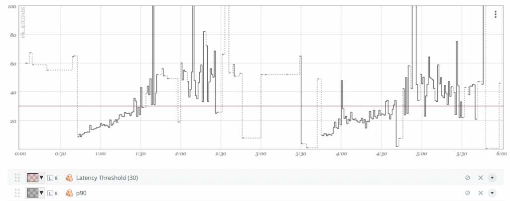
This graph is calculating the 90th percentile over a rolling one-minute period, and you can see it bounces around quite a bit. Although aggregating percentiles is tempting, it can produce materially wrong results — especially if your load is highly volatile.

Percentile metrics do not allow you to implement accurate Service Level Objectives that are formulated against hours or weeks. There are a considerable number of operational time series data monitoring systems, both open source and commercial, that will happily store percentiles at five-minute (or similar) intervals. But the percentiles are averaged to fit the number of pixels in the time windows on the graph, and that averaged data is mathematically wrong.

Percentiles are a staple tool of real systems monitoring, but their limitations should be understood. Because percentiles are provided by nearly every monitoring and observability toolset without limitations on their usage, they can be applied to SLO analyses easily without the operator needing to understand the consequences of how they are applied.

Rethinking How to Compute SLO Latency: Histograms

So what’s the right way to compute SLO latencies? As your services get larger and you’re handling more requests, it gets hard to do the math in real-time because there’s so much data — and it’s not always easy to store. Say you want to calculate the 99th percentile and then decide later, for example, that the 99th percentile wasn’t right — the 95th percentile is. You have to look at past logs and recalculate everything. And those logs can be expensive, not only to do the math on but to store in the first place.

A better approach than storing percentiles is to store the source sample data in a manner that is more efficient than storing single samples, but still able to produce statistically significant aggregates. Enter histograms. Histograms are the most accurate, fast and inexpensive way to compute SLO latencies. A histogram is a representation of the distribution of a continuous variable, in which the entire range of values is divided into a series of intervals (or “bins”) and the representation displays how many values fall into each bin. Histograms are ideal for SLO analysis — or any high-frequency, high-volume data — because they allow you to store the complete distribution of data at scale, rather than store a handful of quantiles. The beauty of using histogram data is that histograms can be aggregated over time, and they can be used to calculate arbitrary percentiles and inverse percentiles on-demand.

For SLO-related data, most practitioners implement open source histogram libraries. There are many implementations out there, but here at Circonus we use the log-linear histogram — specifically OpenHistogram. It provides a mix of storage efficiency and statistical accuracy. Worst-case errors at single-digit sample sizes are 5%, quite a bit better than the hundreds percent seen by averaging percentiles. Some analysts use approximate histograms, such as t-digest. However, those implementations often exhibit double-digit error rates near median values. With any histogram-based implementation, there will always be some level of error, but implementations such as log-linear can generally minimize that error to well under 1%, particularly with large numbers of samples.

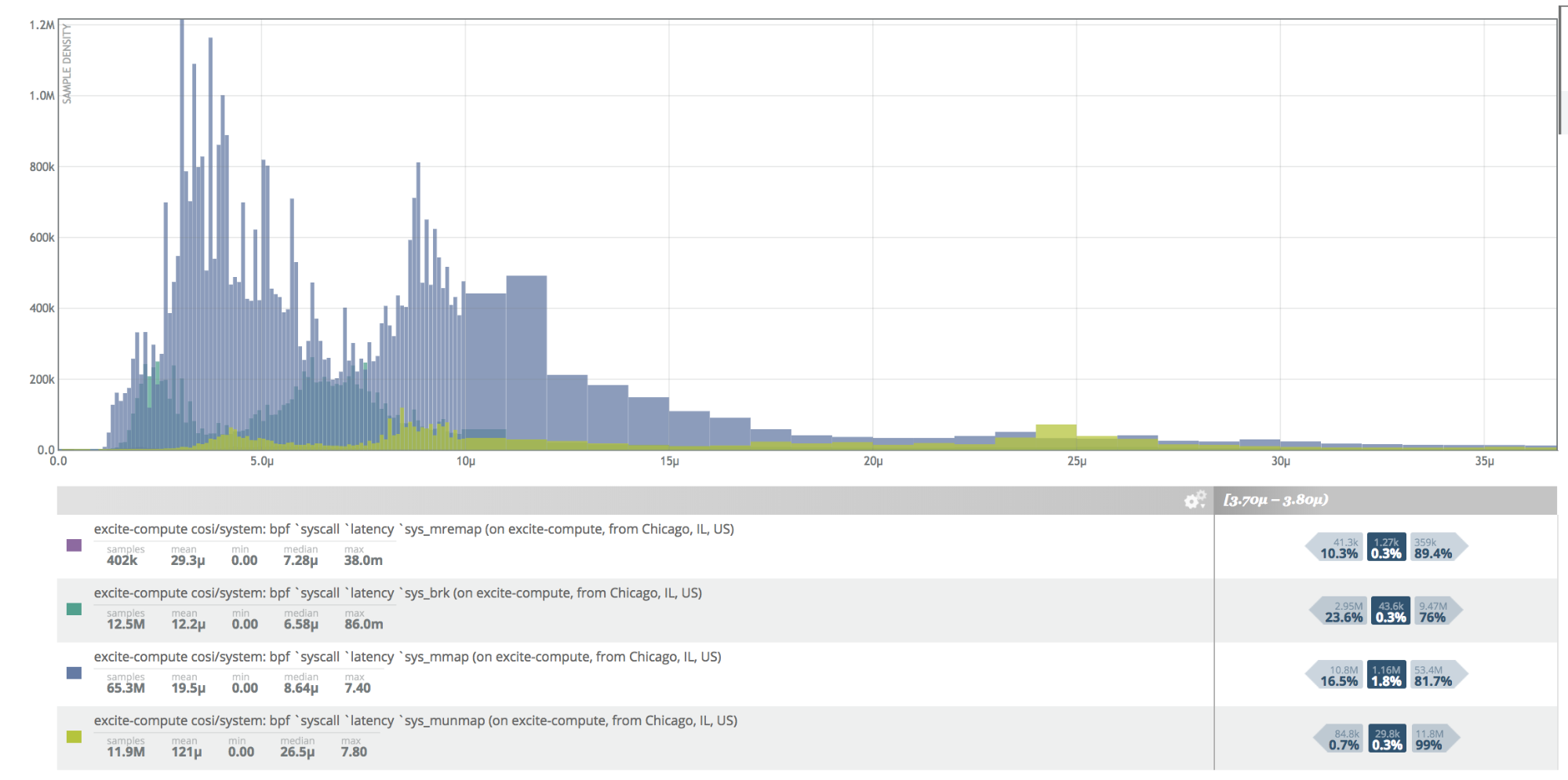
This histogram above includes every single sample that has come in for a specific latency distribution — 6 million latency samples in total. It shows, for example, that 1 million samples fall within the 370,000 to 380,000-microsecond bin, and that 99% of latency samples are faster than 1.2 million microseconds. It can store all these samples at 600 bytes and accurately calculate percentiles and inverse percentiles while being very inexpensive to store, analyze and recall.

Let’s dive deeper into the benefits of histograms and how to use them to correctly calculate SLOs.

Histograms Easily Calculate Arbitrary Percentiles and Inverse Percentiles

Framing SLOs as percentiles is backward — they must be framed as inverse percentiles. For example, when you say “99% of home page requests should be faster than 100 milliseconds,” the 99th percentile for latency just tells us how slow the experience is for the 99th percentile of users. This is not super helpful. What’s more relevant is to know what percentage of users are meeting or exceeding your goal of 100 milliseconds. And when you do the math on that, this is called an inverse percentile.

Also, when framing SLOs, there are two times that are critical:

1. The period over which you calculate your percentile. Example: five minutes.
2. The period over which you calculate your objective success. Example: 28 days.

The reason you need a period over which to calculate your percentile is that looking at every single request over 28 days is difficult, especially considering traffic spikes. So what engineers do is look at these requests in reasonably sized windows — five minutes in this example. So you’ll want to ensure your home page requests are under 100 milliseconds over 28 days, and you’ll look at this in five-minute windows. You’ll have 288 five-minute windows for 28 days and look within each window to ensure that 99% of requests are faster than 100 milliseconds. At the end of 28 days, you’ll know how many windows are winners vs. losers and based on that data, make adjustments as needed.

Thus, stating an SLO as 99% under 100 milliseconds is incomplete. A correct SLO is:

• 99% under 100 milliseconds over any five-minute period AND 99% of those are satisfied in a rolling 28 day period.

The inverse percentile for this SLO is: 99% of home page requests in the past 28 days served in < 100ms; % requests = count_below(100ms) / total_count * 100; ex: 99.484 percent faster than 100ms

These inverse percentiles are easy to calculate with histograms. And a key benefit is that the histogram allows you to calculate an arbitrary set of percentiles — the median, the 90th, 95th, 99th percentile — after the fact. Having this flexibility comes in handy when you are still evaluating your service, and are not ready to commit yourself to a latency threshold just yet.

Histograms Have Bin Boundaries to Ease Analysis

Histograms divide all actual sample data into a series of intervals called bins. Bins allow engineers to do statistics and reasoning about the behavior of something without looking at every single data point. What’s absolutely critical for accurate analysis is that your histograms ensure a high number of bins and that you set your bins the same across all of your histograms.

There are various monitoring solutions available that have histograms, but their number of bins are many times extremely limiting — they can be as low as 8 or 10. And with that number of bins, your error margin on calculations is astronomical. For comparison, Circhlist has 43,000 bins. It’s critical that you have enough bins in the latency range that are relevant for your percentiles (e.g. 5%). In this way, you can guarantee 5% accuracy on all percentiles, no matter how the data is distributed.

It’s important that you set your bin boundary to the actual question you’re answering. So in our example, if you want requests to be faster than 100 milliseconds, make sure one of your bin boundaries is on a hundred milliseconds. This way, you can actually accurately answer the inverse percentile question of 100 milliseconds, because the histogram is counting everything and it’s counting everything less than 100 milliseconds.

Also, your histograms should have common bin boundaries, so that you can easily add all of your histograms together. For example, you can take all histograms from this minute and last minute and add them up into a minute histogram — similarly for hours, days, months. And when you want to know what your 99% was for last month, you can immediately get your answer. In fact, it’s usually a good idea to mandate the bin boundaries for your whole organization, otherwise, you will not be able to aggregate histograms from different services.

Histograms Let You Iterate SLOs Continuously

As a reminder, SLOs should be the lowest possible objective — it’s the minimum your users expect from you — so that you can take more risks. If you set your objective to 99, but nobody notices a problem until you hit 95, then your SLO is too high, costing you unnecessary time and money. But if you set it at 95, then you have more budget and room to take risks. Thus, it’s important to set SLOs at the minimum viable, so you can budget around it. There are big differences between 99.5% and 99.2% and 100 vs 115 milliseconds.

But how do you know what number this should be to start? The answer is you don’t. It’s impossible to get it right the first time. You must keep testing and measuring. By keeping historical accuracy with high granularity via histograms, you can iteratively optimize your parameters. You will be able to look at all of your data together and quantitatively circle in on a good number. You can look at the last two or three months of data to identify at what threshold you begin to see a negative impact downstream.

For instance, the above histogram includes 10 million latency samples, stored every five minutes. This shows how the behavior of your system changes over time and can help to inform you on how to set your SLO thresholds. You can identify, for example, that you failed your SLO of 99% less than 100 milliseconds and were serving requests at 300 milliseconds for an entire day — but the downstream consumers of your service never noticed. This is an indication that you are overachieving, which you should not do with SLOs.

Your software and your consumers are always changing, and that’s why setting and measuring your SLOs must be an iterative process. We’ve seen companies spend thousands of dollars and waste significant resources trying to achieve an objective that was entirely unnecessary because they didn’t iteratively go back and do the math to make sure that their objectives were set reasonably. So, be sure to respect the accuracy and mathematics around how you calculate your SLOs — because they almost directly feed back into budgets. And you can get a bigger budget by setting your expectations as low as possible, while still achieving the optimal outcome.

Respect the Math

When you set an SLO, you’re making a promise to the rest of the organization; and typically there are hiring, resource, capital, and operational expense decisions built around that. This is why it’s absolutely critical to frame and calculate your SLOs correctly. Auditable, measurable data is the cornerstone of setting and meeting your SLOs; and while this is complicated, it is absolutely worth the effort to get right. Remember, never aggregate percentiles. Log-linear histograms are the most efficient way to accurately compute latency SLOs, allowing you to arbitrarily calculate inverse percentiles, iterate over time, and quickly and inexpensively go back to your data at any time to answer any question.

Feature image via Pixabay.